The SID Chip Is a Reservoir Computer

This is the C64 I’ve had since I was a kid. A 1984 breadbin with a working 6581 SID, one of the many Commodores in the house these days, but this is the one I grew up with. I hooked it to my laptop over a serial cartridge, fed a chaotic signal into the SID’s filter (the Lorenz system, the one that gave us the butterfly effect), recorded what came out of the audio jack, and trained a single layer of linear regression to forecast that signal from the chip’s sound.

It spent a couple of afternoons forecasting chaos for this.
It half worked, in a specific and interesting way. Ask it to predict the signal one or two steps ahead and a plain linear model crushes it. Ask it to predict ten or twenty steps ahead, where the chaos has outrun anything a straight line can do, and the forty-year-old sound chip pulls ahead. The 6581 was doing real machine learning in the regime where it’s actually hard.
That’s possible because of a oldish idea called reservoir computing: you don’t have to train a system’s dynamics to compute with it. You just have to train the readout.
Here’s my log of the build, false starts and all
How reservoir computing works
We need three ideas to follow the rest of this: what a reservoir is, why training only the readout works, and where the trick came from.
The three properties
A reservoir is a dynamical system, anything whose configuration changes over time according to some rule. To compute with it, it needs three properties.
State is whatever you need to know about the system right now to predict what it will do next. For a pendulum, that’s the angle and the angular velocity. For an RC circuit, it’s the voltage on the capacitor. The state is the system’s compressed memory of its past.
Nonlinearity means the response to A and B together isn’t the sum of the responses to each alone. Two signals fed in together interact, mix, and fold. Linear systems can only rearrange information. Nonlinear ones create new information. Multiply two tones, and you get the sum and difference frequencies that were in neither input, which is the kind of move a linear system can’t make.
Fading memory means the present state depends on past inputs, with older inputs mattering less. Nudge the input to an RC circuit, and the capacitor voltage traces where the input has recently been. Without memory, you can’t pull out anything that depends on time.
Put all three together, a nonlinear dynamical system with state and fading memory, and you’ve got a reservoir.
The trick
Say you’ve got a signal that wanders around in a complicated way over time, a stretch of speech, a sensor feed, the wiggle of a stock, and you want to guess where it’s going next. The usual tool is a recurrent neural network, a network with loops that can retain a memory of what it just saw. Training one is famously miserable. The error signal has to crawl backward through dozens or hundreds of time steps, getting multiplied at every one, so it either fades to nothing or blows up. Half the deep-learning zoo, the LSTMs and the gated contraptions, exists to dance around that one problem.
Reservoir computing is different. You don’t train the recurrent weights at all. You pick them randomly, freeze them, and train a single linear layer to read out the state.
That’s it.
If your first reaction is “that can’t work,” you’re in good company.
Each entry of the reservoir’s state is some random nonlinear function of the recent input. A random nonlinear function still carries information about its input. Stack a few hundred of them, and the state at any moment is a high-dimensional pile of features pulled from recent history. Some of those features, by luck, line up with whatever you’re trying to predict. Finding the right linear combination is just regression, a closed-form least-squares solve. No backpropagation, one matrix solve.
Similar is the kernel methods. Project your data into a high-dimensional space where the problem becomes linear, then use a linear model there.
Reservoir computing is different. You project the input’s history into a high-dimensional state trajectory, and read it out with a line.
The reservoir has to sit near the edge of chaos. Too damped, and the state forgets the input in a couple of steps. Too explosive and tiny perturbations blow up into wildly different trajectories, and you lose all reproducibility. The sweet spot in between is the echo state property, and it’s exactly what we’ll be tuning the SID’s filter for.
Where it came from
The trick got discovered twice, independently, in 2001 and 2002.
Herbert Jaeger, working on engineering recurrent nets, called his version Echo State Networks and, in a 2004 Science paper, showed that one with about 1,000 reservoir neurons could predict the Mackey-Glass time series 84 steps ahead with roughly two and a half orders of magnitude less error than the prior best.
Wolfgang Maass, working on cortical microcircuits, called his version Liquid State Machines and argued that a generic recurrent population of spiking neurons already has universal power on time series. The cortex doesn’t need to be specially wired to be useful, his version goes. It just needs to be rich enough that downstream neurons can learn to read out whatever they need.
Two people, different fields, different math, same answer within a year. That’s a good sign we’re on to something.
And the substrate doesn’t have to be neurons. It just needs the three properties and the echo state property. In 2003, Chrisantha Fernando and Sampsa Sojakka built a reservoir out of an actual bucket of water, poked the surface with a motor, and trained a linear readout on camera pixels. The water did XOR and classified spoken digits. Since then, people have built physical reservoirs from photonic loops, soft robot bodies, memristors, and cultured neurons. The substrate is swappable.
Which is how a 1980’s sound chip gets on the menu.
The SID as a reservoir
The MOS 6581 was designed in 1982 for the C64. It’s an analog-digital hybrid: digital control logic, real analog filtering, real analog mixing. That hybrid nature is what makes it a credible reservoir.
It has three voices, each with an oscillator (sawtooth, triangle, pulse, or noise) and an envelope, and any subset of them can be routed through one shared analog filter with low-pass, band-pass, and high-pass modes. For our purposes, the filter is the only part that matters.
The filter
The 6581’s filter is a state-variable filter, a textbook circuit that gives you low-pass, band-pass, and high-pass from the same internal state. That state is real and analog, the voltages on two integrating capacitors evolving continuously. That’s the internal memory a reservoir needs.
Cutoff is set by an 11-bit register pair (low 3 bits at $d415, high 8 at $d416, so 2048 values) spanning roughly 30 Hz to 12 kHz. The exact mapping is famously chip-dependent because every 6581 came off the line with slightly different filter behavior due to variations in the on-die capacitors and transistors. This is the part where 6581 owners get philosophical. It’s also exactly what we want: a rich, idiosyncratic, hard-to-predict response.
Resonance is a 4-bit value (high nibble of $d417). Crank it, and the filter behaves like a lightly damped resonator, ringing around the cutoff frequency and decaying over a few milliseconds. That ringing is tunable memory.
The 6581’s filter is nonlinear. The latter 8580 swapped in a cleaner, more linear design, which is why 8580 machines sound tidier and less characterful. For musicians, the 6581’s nonlinearity is characteristic. For a reservoir, it’s the reason to use the chip. A perfectly linear filter can’t make features that a linear readout couldn’t already pull from the input.
Finding a configuration that actually does anything
My first instinct was the showy setup: voice 1 as a triangle, ring-modulated by voice 3, run through a high-resonance band-pass with the cutoff tracking the input. Ring modulation multiplies two signals; multiplication is the canonical nonlinear move, and it sounds like science fiction. On paper, it’s perfect.
In practice, it was dead. I drove the cutoff with the input and measured how well the resulting audio could reconstruct the input, and the answer was: not at all, no better than guessing the average. A triangle wave is nearly all fundamental with weak harmonics, so when you sweep a band-pass across it, there’s almost nothing up there for the filter to grab. The chip made noise, but the noise barely depended on the input.
So I swept configurations. Different waveforms, different filter modes, different voice frequencies and resonances, ten setups in a row, scoring each one by how much the input survived into the audio. The winner, by a clear margin, was a 50% pulse wave through a maximum-resonance low-pass at around 125 Hz. A pulse is harmonically dense, all the way up the spectrum, so when the resonant low-pass sweeps with the cutoff, it carves a moving, input-dependent shape out of a signal that’s rich enough to carve. The old triangle/band-pass setup scored a flat 1.0 (useless). The pulse/low-pass scored well under that, meaning the input was genuinely making it through the filter and into the sound.
That’s the reservoir, in five register writes:
voice 1   : 50% pulse, gated, ~125 Hz   ($d404 = $41)
filter    : voice 1 in, max resonance     ($d417 = $f1)
mode      : low-pass, volume 15           ($d418 = $1f)
cutoff    : driven by the input, 60 Hz     ($d415/$d416)
A harmonically loud oscillator is dragged through a resonant low-pass whose corner frequency is the input. The audio coming out is a nonlinear, memory-laden function of where the input has recently been. That’s a reservoir.
The rig
The hardware:
- The 1984 C64, NTSC, with its original 6581.
- A GGLABS GLINK232 serial cartridge in the expansion port, jumpered to NMI /
$de00so the UART lands where the driver expects it. Running 38400 baud. - An SD2IEC to load the driver.
- An FTDI USB-serial adapter from the cartridge to the laptop.
- The C64’s video and audio into a RetroTink 5X, then into the laptop over HDMI capture.
The flow is simpler than the per-frame chatter I started with. The laptop generates the entire input sequence up front, ships it to the C64 in one burst, and the C64 plays it back vblank-locked at 60 Hz while I record the audio. The serial link is nowhere near the timing loop, so it doesn’t matter how slow it is. Each frame, the C64 writes the next cutoff value to the filter, holds it for one video frame, and moves on. The C64 screen shows a title, a status word for each phase, and a bar that jumps around with the filter cutoff, with the border flipping colors as it works, so I could see what the chip was doing at a glance.
Turning audio into a state vector
We can’t read the filter’s analog state directly. All we get is what comes out of the audio jack. That turns out to be enough, by way of a result from Floris Takens in 1981: you can reconstruct a system’s state space from time-delayed copies of a single observable. The current sound carries some information about the hidden filter state, an earlier slice carries different information, and stacked together they triangulate it.
My first attempt at the features was wrong, and wrong. I took the raw audio energy per frame, the loudness, figuring the filter would get louder and quieter as the cutoff swept. It barely moved. A resonant low-pass doesn’t change how loud a pulse is so much as which harmonics survive, so the energy is roughly flat while the timbre changes completely. The information is in the spectrum, not the volume.
So for each 60 Hz frame, I took the slice of audio recorded during it, run a short FFT, and bin it into twelve log-spaced bands from 200 Hz to 12 kHz. Those twelve numbers are the filter’s spectral fingerprint for that frame, which is to say a fingerprint of the cutoff value that produced it. Then, because memory is the entire point of a reservoir, I stack each frame together with the twenty frames before it. That gives the linear readout a window of recent history to work with, which is where the long-horizon prediction comes from.
Training the readout: ridge regression
The readout is the only thing that gets trained, and it’s the simplest part. For every frame, we have a state vector (the spectral bands, stacked with recent history) and a target (the input value some number of frames in the future). We want a linear combination of state entries that predicts the target. That’s least squares.
Plain least squares blows up when the state dimensions are highly correlated, which they always are here, since neighboring frequency bands and neighboring frames look alike. The fix is ridge regression, least squares with a penalty on large weights:
w = (XᵀX + αI)⁻¹ Xᵀy
The α sets how hard you lean on the penalty. Zero gives you plain least squares and probably overfitting. Large pushes the weights toward zero, underfitting. I grid-search it on a validation split and report error on a separate held-out test split, so nothing I quote is data the model trained on. Seventy percent to fit, fifteen to pick α, and fifteen held out. scikit-learn’s Ridge solves.
Does it beat zero? A chaotic signal like the one I’m feeding in is partly predictable from its own recent values, so I run the exact same regression on the raw input history with no SID at all, same amount of memory. If the SID reservoir can’t beat that, the filter isn’t earning its keep. I also check against just predicting the last value, and against predicting the average.
Forecasting a chaotic system
I gave it is forecasting: guessing where a chaotic signal is headed. That’s what reservoir computing is used for out in the world: predicting things whose dynamics are nonlinear and that straight-line extrapolation can’t see past, like laser intensity, plasma, turbulence, or irregular physiological rhythms.
I picked the Lorenz system, Edward Lorenz’s 1963 model of atmospheric convection and the birthplace of the butterfly effect. It’s the canonical chaotic system: deterministic, bounded, and notoriously unpredictable far out, because two nearly identical starting points diverge exponentially. Its x coordinate drifts back and forth between two lobes, smooth from one moment to the next, but never repeating. I feed that coordinate in as the filter cutoff and ask the readout to predict it some number of frames ahead. Smooth enough that the filter can follow it, chaotic enough that a linear model is helpless past a few steps. Right in the chip’s lane.
Results
One continuous run: 8192 frames took about 137 seconds, the entire Lorenz signal played through the SID once and recorded. Then I trained the readout to forecast different distances into the future and compared it against a linear model handed the same input history.
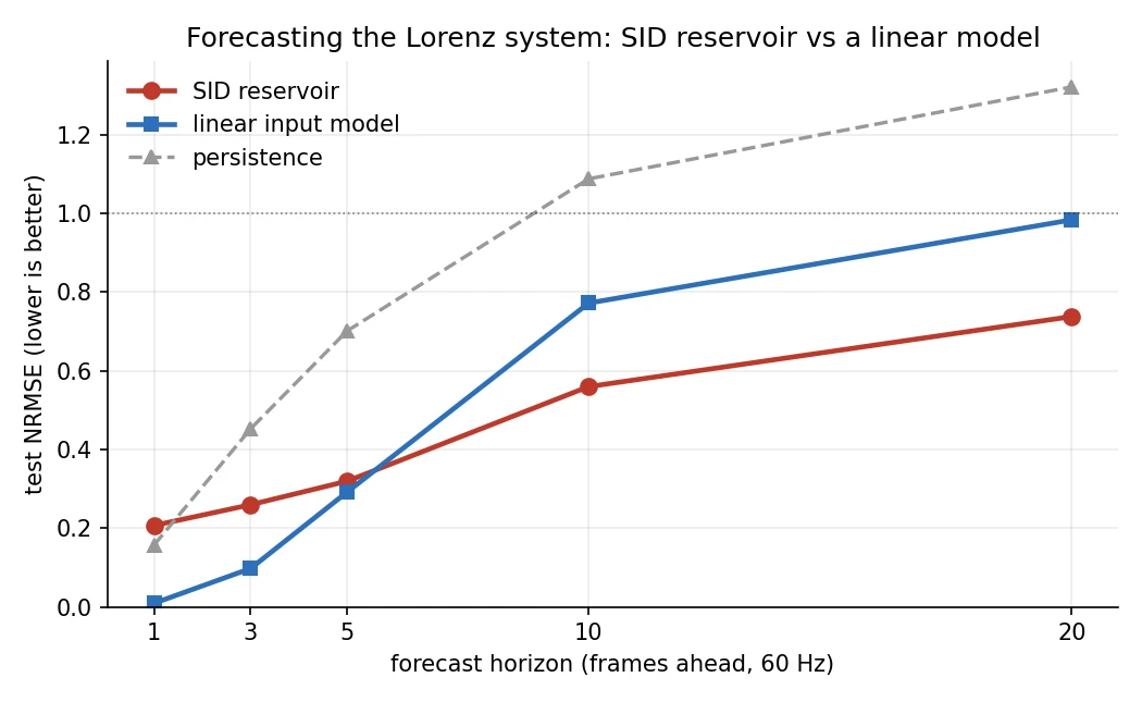
Forecast error against how far ahead you predict the Lorenz system. Lower is better. The linear model works well on short horizons but then falls apart. The SID reservoir takes over once prediction gets genuinely hard.
Test NRMSE, lower is better, where 1.0 is the score you’d get by always guessing the mean:
horizon   SID reservoir   linear input   persistence
   1          0.21            0.01           0.16
   5          0.32            0.29           0.70
  10          0.56            0.77           1.09
  20          0.74            0.98           1.32
Watch the handoff. One step ahead, the linear model is nearly perfect (0.01), because the signal barely moves frame to frame, and the SID’s extra machinery is just noise on an easy job. Five steps, still a linear win, barely. By ten, the straight-line extrapolation is coming apart (0.77), and the SID is comfortably ahead (0.56). By twenty, the linear model is finished, 0.98, no better than guessing the average, while the SID is still carrying real information at 0.74. Lorenz is more violently chaotic than most benchmarks, so the linear model gives up quickly, making the gap stark.
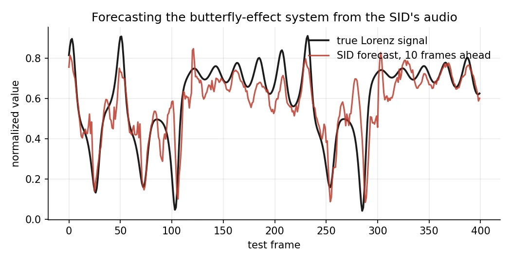
True Lorenz signal in black, the SID’s ten-frames-ahead forecast in red, on held-out test data. It follows the wander between lobes and the deep dips, missing mostly on the fast reversals.
That crossover is the point, and it’s what the theory says should happen: the filter supplies nonlinear memory a linear model can’t fake, and it earns its keep right where straight-line prediction falls apart. It isn’t beating a real echo state network, and it was never going to. It’s a 1982 sound chip forecasting the butterfly-effect system further than a line can reach.
To make sure this wasn’t a quirk of one system, I ran the same setup on Mackey-Glass, the other standard reservoir benchmark (a 1977 model of blood-cell production, chaotic and smooth like Lorenz but gentler). Linear wins the first few steps, the SID takes over by horizon ten and holds through twenty. On a cleaner 96 kHz capture, the ten-step error dropped to about 0.19 against the linear model’s 0.54. Two different chaotic systems, same handoff, so the effect is real and not a fluke of how Lorenz happens to wiggle.
So what’s a chip-as-reservoir good for?
Forecasting a chaotic system isn’t a toy problem. It’s what reservoir computing is used for most. The deeper reason the idea has legs, though, is that one reservoir handles a pile of different jobs, and switching jobs only means retraining the little linear readout on top. The dynamics never change. You fit a new regression, and you’re done.
A few of the things people use physical reservoirs for are:
- Recognizing spoken words. The water bucket classified spoken digits, and it’s the canonical demo because speech is exactly the kind of messy, time-stretched signal a reservoir handles well. Audio in, “which word” out.
- Cleaning up a smeared signal. Jaeger’s original echo state network result wasn’t a toy at all. It was channel equalization, undoing the distortion that a noisy communication line smears across a transmission. That’s a real, shipped use of the trick.
- Noticing when something’s off. Run a sensor stream (a motor’s vibration, a heartbeat, the hum on a power line) through the reservoir and train the readout to predict the next step. When reality no longer matches the prediction, something has changed. That’s anomaly detection without hand-writing a model of “normal.”
- Guessing the near future of a wiggly thing. The Lorenz forecast up top is exactly this, and it’s what reservoirs get pointed at for real chaotic signals.
There’s a catch, though. The input has to drift slowly enough that the filter can follow it from one frame to the next. That’s why predicting a smooth chaotic signal suits this chip, and why anything that flips to a brand-new value every single frame, like a raw symbol stream, is past what a 60 Hz filter sweep can track. Inside that lane, the pitch holds: one physical reservoir, many jobs, only the regression changes. Outside it, you want a faster reservoir than a 1982 sound chip clocked to a TV frame.
And the substrate keeps getting stranger. People have built reservoirs out of spintronic nano-oscillators, tangles of optical fiber, FPGA delay loops, the flex of a soft robot’s body, and arrays of memristors. The SID is just an unusually charming entry on that list. The most literal entry, though, is biological, and that’s the thread this whole project hangs off.
What this means: the bridge to brain-inspired computing
Reservoir computing is having a moment, not because anyone’s shipping a SID-based fraud detector, but because the core instinct, don’t optimize the substrate, optimize the readout, keeps reappearing in the parts of computing that are trying to look more like brains.
Liquid State Machines, the cortical version of this trick, backs a school of neuroscience that says the cortex isn’t specially designed for any one task. It’s a big, rich, recurrent system, and downstream regions learn linear-ish readouts off it. Spiking networks and neuromorphic chips like Loihi and SpiNNaker all lean on recurrent populations of nonlinear units with built-in memory, training mostly at the readout. The reservoir intuition is the scaffolding, even when nobody names it.
Then there’s the Biological Processing Unit thread, which is what got me down this whole road in the first place. I wrote earlier about biological processing units on this same Commodore 64, running a fruit fly’s odor-hashing trick on plain 6502 hardware, and I’ve been working through a full reproduction of the paper it’s based on since (with curious results). The SID piece is the same instinct from the other direction: instead of borrowing a brain’s algorithm and running it on silicon, borrow a chip’s dynamics and read them out like they were a brain. BPUs, in recent work from Joshua Vogelstein and colleagues, push the idea all the way: build computational substrates that aren’t digital models of brains but actual biological tissue, cultured neurons, organoids, slices of cortex wired to electronics. The reasoning is the reservoir reasoning, just bolder. If the substrate doesn’t have to be trained, and biological substrates are already absurdly rich at the dynamics that matter, then maybe the right computer for some problems is a literal dish of cells.
Computing the substrate doesn’t have to be the hard part. The hard part can be just the readout. A twenty-five-year-old idea that keeps re-arriving with a new substrate. A recurrent net, a tank of water, a soft robot’s arm, a 1982 sound chip, a cluster of cultured neurons.
The C64 isn’t an answer to anything. It’s an existence proof, and just a fun way to explore the idea. A machine that mostly played games just forecast a weather-like chaotic system, at horizons a linear model can’t reach, with a single matrix solve. If a sound chip can do that when you treat it right, it makes you wonder what the next forty years look like once we stop assuming the substrate has to be silicon and trainable. That’s the question the BPU work is taking seriously, and it’s why this wasn’t only a weekend with an old computer. I got to hear the thing sing while it did it.
References
- Jaeger, H. (2001). The “echo state” approach to analyzing and training recurrent neural networks. GMD Report 148.
- Jaeger, H. & Haas, H. (2004). Harnessing nonlinearity: Predicting chaotic systems and saving energy in wireless communication. Science, 304(5667), 78-80.
- Maass, W., Natschläger, T., & Markram, H. (2002). Real-time computing without stable states. Neural Computation, 14(11), 2531-2560.
- Fernando, C. & Sojakka, S. (2003). Pattern recognition in a bucket. ECAL 2003.
- Tanaka, G. et al. (2019). Recent advances in physical reservoir computing: A review. Neural Networks, 115, 100-123.
- Lukoševičius, M. (2012). A practical guide to applying echo state networks. Neural Networks: Tricks of the Trade, 2nd ed.
- Mackey, M. C. & Glass, L. (1977). Oscillation and chaos in physiological control systems. Science, 197(4300), 287-289.
- Takens, F. (1981). Detecting strange attractors in turbulence. Lecture Notes in Mathematics, vol. 898, Springer.